← worksCourse project · Intelligent robotics2025
Reactive Robots using ROS2 and Webots
Memory-less wall following and robot tracking in Webots, contrasting proximity-only control against LiDAR-based RANSAC circle fitting.
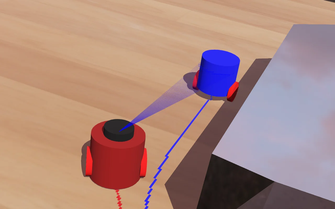
With Félix Martins, Francisco da Ana and Martim Iglesias · Topics in Intelligent Robotics, FEUP
Two differential-drive robots navigate a question-mark-shaped arena with zero memory, maps, or global coordinates. One robot tracks the perimeter wall; a faster follower tracks either the wall or the lead robot. A minimalist baseline relying purely on infrared proximity sensors navigates outer bends smoothly, but collides catastrophically inside the interior concavity where wall reflections and robot silhouettes blur together. Adding a 2D planar LiDAR with spatial clustering and RANSAC circle fitting lets the follower isolate the leader's 4.5 cm cylindrical chassis, dynamically halt within 35 cm, and eliminate deadlock in confined spaces.
The environment & reactive constraints
The arena is a question-mark-shaped obstacle modeled in Blender and imported into Webots with rigid-body collision surfaces and physical contact properties.
Unlike trivial rectangular arenas or endless convex loops, a question mark introduces three distinct navigation challenges:
- Extended straightaways where wall-following controllers accumulate lateral drift.
- Sharp convex corners that break sensor contact and risk unconstrained outward spiral turns.
- A narrow interior concavity (the hook of the question mark) where boundary surfaces converge from multiple angles, severely restricting maneuverability.
The experimental setup enforces purely reactive control, following the behavior-based robotics paradigms of Brooks and Arkin. The robots maintain zero state across control cycles: no SLAM, no odometry accumulation, no occupancy grids, and no inter-robot communication. At each sensor callback, the control node computes linear and angular velocity commands (v, ω) exclusively from instantaneous measurements.
To make interactions dynamic, the follower runs at a higher linear velocity than the leader (0.07 m/s vs. 0.06 m/s). At matching velocities, two robots starting at an offset would maintain static separation, never testing collision avoidance or tight-corner queueing.
Phase 1: the proximity-only baseline
The baseline implementation equips both robots with identical sensing suites: two directional infrared proximity sensors mounted laterally (left and right), with a maximum measurement range of 0.15 m.
Control law
The wall follower executes a proportional steering law relative to a target setpoint threshold:
d_thresh = 0.9 · MAX_RANGE = 0.135 m
At each sensor update:
- If
d_right < d_thresh(too close to the wall), steer counter-clockwise away:ω = +1.5 rad/s. - If
d_right > d_thresh(too far from the wall), steer clockwise toward the wall:ω = v_cur · ω_def / v_def = -0.45 rad/s.
The robot-follower applies an identical rule to whatever obstacle enters its proximity cone, treating a peer robot identically to a stationary wall.
Loop time dynamics
Loop completion time scales inversely with linear velocity. Increasing v from 0.06 m/s to 0.12 m/s almost exactly halves the circuit duration, confirming that the reactive steering law maintains trajectory geometry across speeds:
| Linear velocity (m/s) | Loop completion time | Trajectory stability |
|---|---|---|
| 0.06 | 2 min 32 s | Stable exterior tracking; occasional corner overshoot |
| 0.08 | 1 min 56 s | Nominal speed; consistent outer perimeter following |
| 0.12 | 1 min 16 s | Aggressive wall corrections; higher oscillation along straightaways |
Failure mode: scalar range ambiguity
The baseline fails predictably inside the central concavity of the question mark. Proximity sensors output a single scalar: distance to the nearest reflective surface. They carry zero geometric information—an echo of 8 cm from a drywall surface is indistinguishable from an echo of 8 cm from a robot chassis.
Along outer walls, the faster follower occasionally overtakes or runs parallel without incident. But once the robots enter the interior hook, the confined corridor forces both robots within sensing distance simultaneously:
- The leader slows down to negotiate the sharp interior corner.
- The faster follower approaches from behind and detects the leader's chassis on its right sensor.
- Interpreting this as an intruding wall, the follower steers hard left—straight into the actual arena wall.
- The left and right sensors simultaneously fire below
d_thresh, producing conflicting steering corrections that wedge both chassis against each other and the obstacle corner, causing permanent deadlock.
Phase 2: LiDAR & RANSAC circle fitting
To resolve the ambiguity without adding memory, the follower was upgraded with a forward-facing 2D planar LiDAR with a fixed 90° horizontal field of view (from −π/4 to +π/4 radians) and a maximum detection range of 0.5 m, providing 360 radial range samples per scan.
Raw LaserScan ranges (360 beams, 90° FOV)
          │
          ▼
Euclidean clustering (split on Δr > 0.20 m)
          │
          ▼
RANSAC circle fitting (100 iterations per cluster)
          │
          ▼
Geometric validation:
  ├── Inliers ≥ 15 (within 0.05 m tolerance)
  └── Fitted radius r ∈ [0.03 m, 0.06 m]
          │
     ┌────┴────────────────────────┐
     ▼                             ▼
[Target detected]           [No target found]
  ├── Proportional steering   └── Fall back to lateral
  │   to circle center            proximity wall-following
  └── Adaptive braking
      (v = 0 if dist < 0.35 m)
1. Spatial clustering
Raw range measurements [r_0, r_1, ..., r_N] are converted to Cartesian points using the beam angle θ_i = θ_min + i · Δθ.
A single-pass Euclidean segmentation divides the scan into distinct candidate clusters whenever consecutive finite beams exhibit a range jump exceeding the spatial discontinuity threshold:
|r_i - r_{i-1}| > 0.20 m
This separates continuous surfaces (such as planar wall segments) from detached obstacles (such as the preceding robot).
2. RANSAC circle estimation
For each cluster containing at least 15 points, RANSAC evaluates up to 100 candidate hypotheses:
- Sample three non-collinear points
(p_a, p_b, p_c)uniformly at random. - Compute the unique circle passing through them, defined by center
(x_c, y_c)and radiusr. - Count inlier points whose orthogonal distance to the circle circumference satisfies
|||p_i - (x_c, y_c)|| - r| ≤ 0.05 m. - Retain the candidate circle maximizing total inliers.
3. Geometric model verification
Walls produce either linear point distributions (where fitted circles yield near-infinite radii) or fragmented clusters with few inliers. A candidate is validated as the target robot if and only if:
inliers ≥ 15 and 0.03 m ≤ r ≤ 0.06 m
Because the physical robot radius is known (r_true = 0.045 m), this constraint filters out flat wall faces, rectangular outer frames, and acute inner corners.
4. Closed-loop pursuit & adaptive braking
Once the leader's position (x_c, y_c) is confirmed, the follower switches its control mode from wall-following to target pursuit:
-
Steering: The bearing angle
θ_target = atan2(y_c, x_c) + π/4sets proportional turning:ω = (θ_target / θ_max) · ω_maxwhereω_max = 1.5 rad/s. -
Adaptive braking: If Euclidean distance
d = sqrt(x_c² + y_c²) < 0.35 m, linear velocity clamps to zero:v = 0ifd < 0.35 m, otherwisev = 0.07 m/s.
When the leader pulls ahead beyond 0.35 m, the follower resumes forward motion. If the leader turns out of the LiDAR's 90° FOV, the algorithm reports zero valid circles, and the follower drops back to proximity wall-following.
Trajectory analysis & results
Each robot was equipped with a virtual pen emitter attached to its center of mass, drawing its continuous ground-truth trajectory on the arena floor (blue for the leader, red for the follower).
The difference between the two systems is visible in the trajectory plots:
- Exterior perimeter: Both architectures track outer convex curves with minimal deviation. The leader maintains a consistent offset from the wall, and the follower tags along smoothly.
- Interior concavity: In the baseline (left), the follower's pen trace diverges wildly from the perimeter. As it attempts to evade the leader, it collides with the inner wall, oscillates between sensors, and halts. In the improved architecture (right), the trajectory remains smooth and strictly parallel across repeated loops.
| Metric | Baseline (proximity only) | Improved (LiDAR + RANSAC) |
|---|---|---|
| Perception modality | 2× Lateral infrared sensors (1D scalar) | 2× Lateral proximity + 2D planar LiDAR (90° FOV) |
| Obstacle discrimination | None (walls and robots share identical echoes) | Geometric (RANSAC circle fitting on cylindrical chassis) |
| Concavity collision rate | 100% (deadlock within 2–3 loops) | 0% (zero collisions across multi-loop runs) |
| Trajectory parallelism | Degrades sharply in confined corners | Uniform across exterior and interior perimeters |
| Queueing behavior | Blind collision avoidance (turns into walls) | Autonomous distance-gated braking at 0.35 m |
Resolving bottlenecks without memory
In a purely reactive agent, spatial coordination cannot rely on reservations or mutual planning. By coupling geometric object recognition with distance-gated halting, the follower queues behind the leader:
- The leader enters the narrow hook and slows during its turn.
- The faster follower detects the leader at 35 cm and halts completely.
- The leader clears the corner and opens distance.
- The follower detects
d > 0.35 m, restarts forward motion, and follows through the bend.
Deadlock is resolved purely through real-time sensory thresholds, with zero memory of previous states.
Failure modes & limitations
The system reveals several fundamental trade-offs inherent to memory-less robotics:
- RANSAC false negatives: To ensure walls are never mistaken for robots, RANSAC thresholds were tuned conservatively (≥ 15 inliers,
r ∈ [0.03, 0.06] m). At acute viewing angles or when the leader is partly clipped by the 90° FOV boundary, the visible arc contains too few points to meet the inlier floor. The follower momentarily loses target lock and reverts to wall-following until the leader re-enters full view. - Initialization sensitivity: The robots must be spawned near a perimeter wall. Because the reactive controller has no global exploration state or wandering schema, spawning in open space far from any obstacle leaves the proximity sensors starved of signal, resulting in open-loop forward drift.
- Discontinuous velocity profiles: Braking is binary (0 m/s or 0.07 m/s). While effective in simulation, real differential drives would suffer high mechanical jerk and wheel slip, requiring a continuous PID distance-error controller with acceleration limits.
