← worksCourse project · Data science202420/20
Predicting Health Insurance
A 72k-row customer dataset where 90% accuracy meant a model that had learned nothing, and the work was all in the two steps before the classifier.
With David Pinto and Francisco da Ana · Introduction to Data Science, FCUP/FEUP
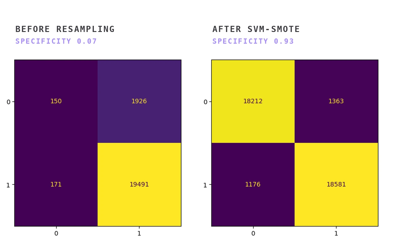
The assignment sets up a scenario: you work as a data scientist for a company, and you have to find which of your customers have no health insurance. The data is customer.csv, 72,458 US customer records across 15 columns covering age, sex, employment, income, marital status, housing, vehicles, gas usage and state of residence, plus a second file of 804 records with the insurance field masked, for a Kaggle leaderboard scored on F1. Only 9.5% of the training customers are uninsured. The first random forest scored 90.4% accuracy and 0.949 F1, and found 150 of the 2,076 uninsured people in its validation split; a model that answers "insured" to everything scores 0.950. Most of the project went into the two steps before the classifier: cleaning columns that hold placeholder values rather than measurements, and rebuilding the class balance.
What the data looks like
72,458 rows, 15 features, no duplicated rows, and 32,260 missing cells (2.97% of the table). The target, health_ins, splits 65,553 insured against 6,905 uninsured.
The signal is real but nowhere near decisive. Employed customers are insured 90.66% of the time against 75.23% for the unemployed. Both homeowner categories sit near 94% insured, renters and rent-free occupants at 84-85%. State of residence spreads wider than either. Alaska (18.75% uninsured), Texas (17.78%) and Georgia (15.20%) sit at one end, Vermont (2.74%), Massachusetts (3.00%) and Hawaii (3.39%) at the other, a sevenfold range.
The missing cells fall into exactly two blocks. is_employed accounts for 25,515 of them on its own. The other 6,745 sit in housing_type, num_vehicles and gas_usage, at 1,686 each, the same number three times, plus 1,687 in recent_move_b. Those four columns go missing together: one block of about 1,686 records missing their household information, not four independent gaps.
Columns that were not what they claimed
age. The column runs from 0 to 120 with a mean of 49.2, which reads like an ordinary long tail until you plot it.
The histogram has a spike at 0, then nothing at all until 21, then the real distribution, then isolated bars at 100, 110, 114 and 120. Binning income and vehicle counts by age band confirms what that implies: the [0, 5) band averages 36,700 in income and 1.95 vehicles, values that belong to a working adult, and the [100, 105) band does the same. 43 rows are aged 0 and flagged employed; 167 are over 90 and flagged employed. Ages outside [21, 99] were therefore set to missing and imputed rather than kept or dropped.
code_column. It is state_of_res in a different alphabet. Cramér's V between the two comes out at exactly 1.0, so one of them goes.
rooms. Its six values are almost perfectly uniform, at 12,042 / 12,230 / 12,134 / 11,955 / 12,098 / 11,999 for one through six rooms, and its Cramér's V against the target is 0.0084.
The health_ins row of that matrix also serves as a leakage check. The strongest categorical association with the target is housing_type at 0.16, followed by marital_status at 0.15. No feature is quietly encoding the answer, and no feature is going to carry a model on its own either.
Missingness as a feature
is_employed is 35.2% missing, and the obvious move is to fill it with False.
The split is 44,630 employed, 2,313 unemployed, 25,515 missing. Filling the blanks with False would have turned a 3.2% unemployment rate into 38.4%, which is not a small distortion of a feature that separates 90.66% from 75.23% on the target. The age profile of the missing rows peaks hard between 66 and 69 and rises again at 21-25, so these are retirees and students. The values are not missing at random, and their absence is itself a signal.
So is_employed was label-encoded with the missing level kept as its own category, then one-hot expanded into three indicators. The model gets employed, unemployed and no record on file as three distinct states. recent_move_b got the opposite treatment (encoded, its missing level restored to NaN, then imputed) because its 1,687 gaps belong to the household block rather than to a population the dataset systematically skips.
The preprocessing pipeline
One function, applied to both the training file and the held-out file, in this order:
| Step | What it does |
|---|---|
| Drop columns | The index, custid, and code_column |
| Clip age | Values outside [21, 99] become NaN |
| Min-max scale | age onto [0, 10]; state_of_res onto [0, 1] once encoded |
| Log-normalise | log1p(x − min + 1) on income and gas_usage |
| Label-encode | sex, is_employed, state_of_res, health_ins |
| One-hot encode | marital_status, housing_type, is_employed |
| Restore NaN | recent_move_b's encoded missing level back to NaN |
| KNN impute | k = 5, distance-weighted, over the whole frame |
Income runs from −6,900 to 1,257,000 against an interquartile range of 41,300, and gas_usage has a median of 10 with a maximum of 570. Both are long right tails that would otherwise dominate any distance-based step, including the imputer that runs immediately afterwards, which is what the log transform is there for. The output is 19 features with zero missing cells.
One thing the pipeline does not do is drop rooms. The EDA concludes it should be dropped and the function never removes it, so all eight models below carry it as a nineteenth feature. At a Cramér's V of 0.008 it is close to inert and the tree-based models will mostly route around it, but it is there.
Why the first round of models was meaningless
Three classifiers on the preprocessed but still imbalanced data, one hyper-parameter each, 70/30 split:
| Model | Accuracy | F1 | Specificity |
|---|---|---|---|
| Decision tree, max_depth 9 | 0.901 | 0.948 | 0.060 |
| Random forest, 100 trees | 0.904 | 0.949 | 0.072 |
| KNN, k = 11 | 0.903 | 0.949 | 0.056 |
A classifier that ignores its input and answers "insured" every time scores 0.904 accuracy and 0.950 F1 on this split. All three tuned models land within half a point of that, and on F1 all three land below it.
In the sweep on the left, specificity is the only line that moves, and it moves downwards: 0.16 at ten trees, 0.07 at five hundred. Everything else is flat, so a sweep scored on accuracy or F1 would have read the 500-tree model as marginally the best one.
This is also where the project's own mid-term checkpoint had landed, concluding that all the models performed similarly across the key metrics and that decision trees and logistic regression were therefore the optimal choices, being cheaper. Both halves of that conclusion are artifacts of the class distribution.
Rebalancing, and picking which rebalancing
Six resampled training sets, built with imbalanced-learn:
| Method | Resulting split | Size |
|---|---|---|
| SMOTE-ENN | 56.5 / 43.5, majority flips | 109,906 |
| SMOTE-Tomek | 50 / 50 | 130,462 |
| Borderline-SMOTE | 50 / 50 | 131,106 |
| SMOTE-ENN then Borderline | 50 / 50 | 124,192 |
| ADASYN | 50.3 / 49.7 | 131,917 |
| SVM-SMOTE | 50 / 50 | 131,106 |
Choosing between them on downstream accuracy would mean fitting models on six datasets and comparing numbers that each carry their own resampling artifacts, so the sets were scored directly instead, with problexity's feature-based complexity measures.
| Dataset | F1 | F2 | F3 | F4 |
|---|---|---|---|---|
| SMOTE-ENN | 0.690 | 0.514 | 0.997 | 0.996 |
| Borderline-SMOTE | 0.760 | 0.514 | 0.997 | 0.996 |
| SMOTE-Tomek | 0.787 | 0.514 | 0.997 | 0.996 |
| SMOTE-ENN + Borderline | 0.744 | 0.514 | 0.997 | 0.996 |
| ADASYN | 0.818 | 0.514 | 0.997 | 0.996 |
| SVM-SMOTE | 0.610 | 0.000 | 0.969 | 0.915 |
problexity normalises every measure so that higher means harder, so SVM-SMOTE is the least complex set on all four axes and the pick follows straight from the table. (The notebook states the criterion the other way round, as "high F1 and low F2", which reads backwards against that normalisation, though it lands on the same dataset either way.)
That zero deserves suspicion. F2 measures the volume of the region where the classes overlap on each feature, and a dataset where they do not overlap at all is an easier problem than the one that was posed. SVM-SMOTE synthesises its minority points from support vectors near the decision boundary, and the resulting set is cleanly separable in a way the original 72,458 records are not. Every score below should be read against that.
The chosen set is 131,106 rows, 65,553 per class.
Eight models on the balanced set
Trees and KNN were swept over a single hyper-parameter. Logistic regression, SVM, XGBoost and the MLP went through GridSearchCV at five folds, scored on F1, which on a balanced set is no longer the metric that was lying earlier.
| Model | Accuracy | Precision | Recall | F1 | Specificity |
|---|---|---|---|---|---|
| Random forest, 100 trees | 0.935 | 0.932 | 0.940 | 0.936 | 0.930 |
| XGBoost, depth 7, lr 0.1, subsample 0.5 | 0.914 | 0.906 | 0.924 | 0.915 | 0.903 |
| KNN, k = 5 | 0.890 | 0.957 | 0.818 | 0.882 | 0.963 |
| Decision tree, max_depth 15 | 0.869 | 0.886 | 0.849 | 0.867 | 0.890 |
| MLP, layers (13, 9, 5), ReLU, Adam | 0.827 | 0.842 | 0.807 | 0.824 | 0.847 |
| SVM, RBF | 0.817 | 0.840 | 0.785 | 0.811 | 0.849 |
| Logistic regression, C = 50, lbfgs | 0.801 | 0.806 | 0.795 | 0.800 | 0.806 |
| Gaussian naive Bayes | 0.767 | 0.773 | 0.757 | 0.765 | 0.776 |
In the earlier round, specificity was a bar one-thirteenth the height of the others. Here every model's five metrics sit within a few points of each other. KNN is the lone exception, and it has swung the other way: the highest specificity in the table at 0.963, bought with the lowest recall at 0.818, now that the minority class has been filled in densely enough for nearest-neighbour voting to favour it.
Random forest at 100 trees wins on four of five metrics with default settings and no grid search. XGBoost, given 27 configurations to search, loses to it by two points; its grid capped max_depth at 7, while the forest's trees grow unconstrained, and a single unpruned tree on this data reaches depth 40. The linear and kernel methods land 12 to 17 points behind the ensembles, and the MLP's grid never offered anything larger than a (13, 9, 5) network, so it was never given the capacity to compete.
The SVM row deserves an asterisk: its parameter grid contains a single candidate (kernel='rbf', fixed seed), so it is the only model in the table that was not actually tuned.
Re-running the forest's tree sweep on the balanced data settles the earlier anomaly. Specificity is now flat across the whole range, moving less than half a point between ten trees and five hundred instead of halving, while accuracy, recall and F1 climb and level off by about seventy-five. The final model is that forest at 100 trees, refit on all 131,106 rows and run over the 804 held-out customers.
Caveats
The pipeline works, and several parts of it would not survive a careful review.
Resampling happens before the split. SVMSMOTE.fit_resample runs on the full X, y, and train_test_split runs on the result. Synthetic minority points are interpolated between real neighbours, and those neighbours land on both sides of the split, so the test half contains points partly constructed from the training half. The 0.935 is optimistic by an unknown margin. The correct order is to split first and resample inside the training fold only. The one comparison this does not touch is the before-and-after contrast with the baseline, since those models never saw a synthetic row.
The target is visible to the imputer. KNNImputer is fitted on the whole training frame, and at that point health_ins is still one of its columns, so a customer's insurance status is one of the coordinates used to find the five neighbours that fill in their age, vehicle count, gas usage and recent move. On the held-out file the target is dropped first, so the imputer there works with different information than the one that produced the training data.
Every transform is refitted on the test file. The scalers, the label encoders and the x − min shift inside the log transform are all fit_transform calls inside a function that also runs on the 804-row test set. A raw age or income therefore maps to whatever those 804 rows imply rather than to what the training set established. With a test file spanning the same range it makes little difference, and it is the kind of thing that fails silently when it does.
The complexity argument cuts both ways. SVM-SMOTE was chosen because it produces the cleanest dataset, and the cleanliness is the part that was manufactured. A 0.93 specificity on a set with zero measured class overlap is not a claim about 0.93 specificity on real customers.
What none of that touches is the finding the project was built on: at this class ratio, accuracy and F1 say almost nothing, and the confusion matrix is where the answer is.
